Home Blog Page 14

Western Sydney Airport Highlights Importance of Technology in Earthworks

Figure 1. Sixteen temporary and four permanent basins with the capacity between 48.1–131 megalitres (12.7 million to 34.6 million gallons) each.

The Western Sydney International (Nancy-Bird Walton) Airport (WSA) project is a rare greenfield opportunity for a new airport rather than a reconstruction or renovation of an existing airport. It is also one of the largest civil earthmoving projects in Australia’s history.

The airport will open in late 2026 and is projected to serve up to 10 million domestic and international passengers annually. The overall design of the terminal and airport property brings together best practices to offer passengers and airlines an experience unrivalled among Australian airports.

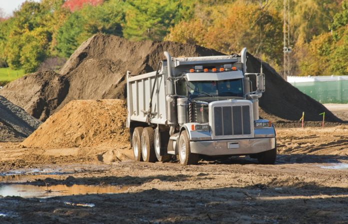
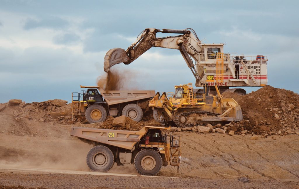
Major earthworks commenced on the project in 2020 and involves moving around 25 million cubic metres (32.7 million cubic yards) of earth to support the construction of the major elements of the airport including the 3.7 km (2.3 mile) runway and the passenger terminal. The earthworks has been conducted in stages, allowing for handover of areas to other contracts to support the construction of the runway and terminal by late 2026.

Other distinctive features of the project’s scale, area and volume include:

  • 470 ha (1,161 acres) topsoil stripping and stockpiling for later reuse in the landscaping phase.
  • 7.3 million square meters (8.7 million square yards) of landscaping.
  • 7,000 lineal metres (4.3 miles) of trunk drainage.
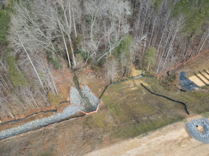
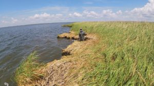
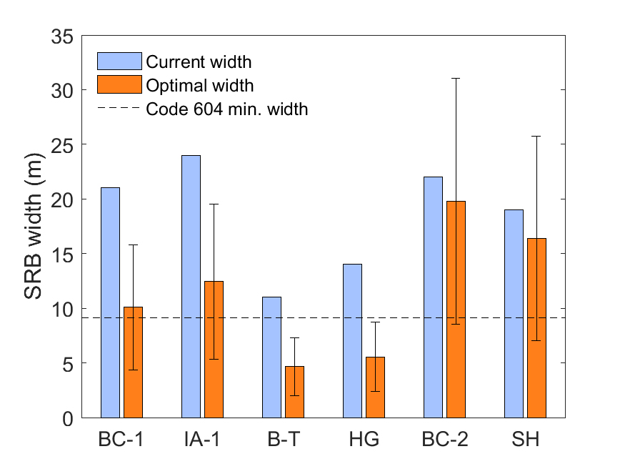
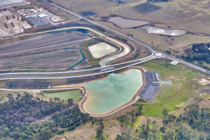
  • Construction of four permanent flood detention and bioretention basins with capacity to control 1:100-year average recurrence interval (ARI) events. These basins have capacity between 48.1–131 megalitres (12.7 million to 34.6 million gallons) each (Figure 1).
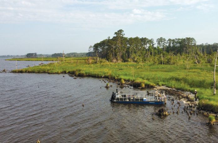
  • 134 potential archaeological sites that required investigation and salvage prior to commencement of construction. The scale of the archaeological program required a team of 138 Aboriginal site officers to assist the project’s archaeologists to investigate and salvage the 134 areas over a period of 12 months. The salvage operation involved wet sieving procedures with 100% recycled water that was not discharged to the environment.
  • 507 threatened plants that were relocated into the airport’s environmental conservation zone prior to construction commencing.

Located on the east coast of Australia, the airport is approximately 41km (25.4 miles) west of Sydney central business district. On average, the area receives a median rainfall of 651.8 mm, with an average of 69.1 days of rain. Since commencement in 2020, the project has been subjected to two consecutive years of La Niña conditions. This has resulted in much greater than average rainfall, with over 1,000 mm of rain received each year, including to date in 2022. This excessive rainfall, accompanied by challenges with COVID-19 has exasperated the risks and challenges involved with such a large-scale project, such as impacts to construction schedule and maintaining compliance with both state and federal regulations. Innovative and dynamic tools and processes to effectively manage the risks involved include:

  • Design and establishment of 16 temporary basins to prevent sedimentation in the surrounding waterways and to protect aquatic life. These basins have the capacity to retain over 400 megalitres (over 160 million gallons) of water.
  • Sediment basin treatment procedures and dewatering logistics to handle the vast quantities of water collected.
  • Sustainable management of silt reuse from basins.
  • Around 99% of water used for construction purposes, including dust suppression, has been obtained from recycled sources and without relying on groundwater, abstraction from rivers or potable water sources. Recycled sources included reuse of water captured during rainfall as well as off site locations.
Figure 2. Comparison of project site as construction progressed.

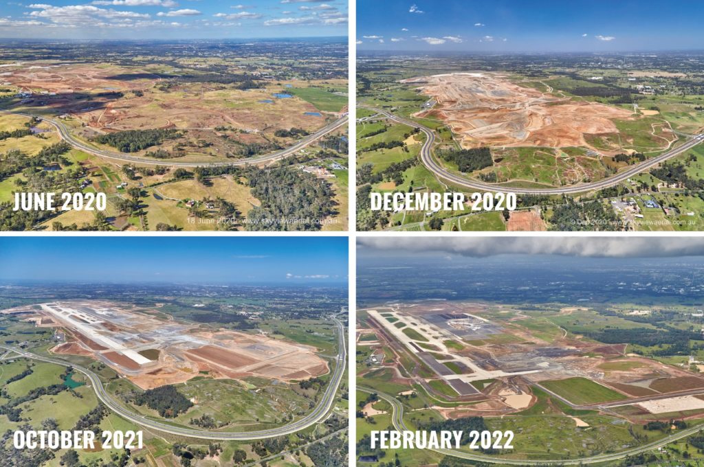
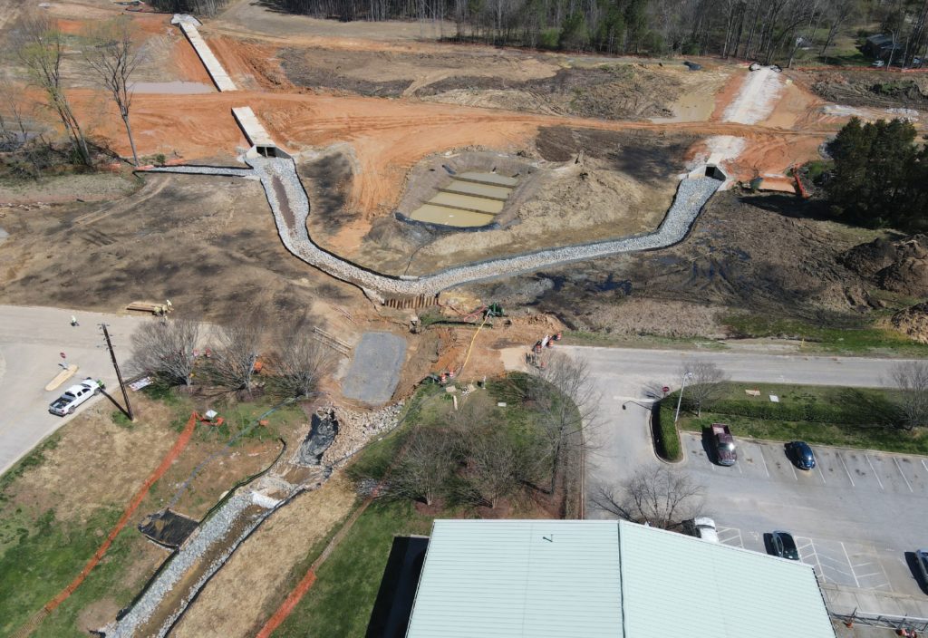
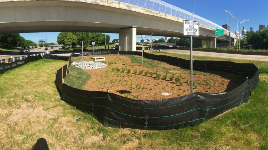
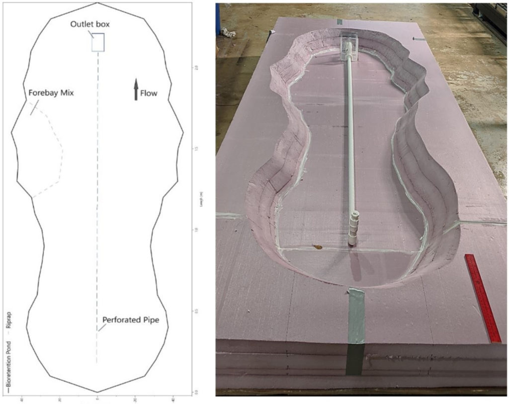
The biggest environmental challenge the construction team faced was the large-scale management of erosion and sediment control in a landscape that was quickly changing as earthworks progressed (Figure 2). With approximately 25 million cubic metres (32.7 cubic yards) of material to be moved at a rate of approximately one million cubic metres (1.3 million cubic yards) every month, the project’s landform and catchments changed at a significant rate (Figure 3). The earthworks program involved the site transitioning from 16 catchments to five over a period of approximately 24 months. For the project to be a success it was critical to have appropriately sized sediment basins in place for every catchment at every stage. This required careful planning of sediment basin sizes, positions and catchment diversions to ensure water run-off from rain events could be appropriately controlled at all times.

One of the key tools the joint venture environment team developed to monitor erosion and sediment control planning compliance was the monthly basin and catchment aerial surveys. Changes in catchments were predicted and forecasted where possible, however due to the dynamic nature of bulk earthworks and different geological conditions encountered it was important for the project team to establish a monthly reporting procedure to self-audit compliance with the site’s erosion control design standards.

The basin aerial reporting process is conducted with these key steps:

Step 1: Monthly aerial LiDAR surveys.

Drones and manned aircraft are used to take aerial LiDAR surveys of the entire site. Due to the size of basin catchments, ground-based surveys are not practical. Catchments average 54 ha (133 acres) but could be up to 327 ha (808 acres).

Step 2: LiDAR data conversion to user friendly GIS platform.

The LiDAR data collected during the surveys is converted to contour and watershed data which is then uploaded onto the project web-based GIS platform. The GIS platform enables all team members to easily access, view and interpret the data.

Step 3: Catchment mapping via GIS review.

Catchments are manually mapped to ensure sub surface drainage structures and pre-rain diversion drainage controls that would not be picked up by the survey data are considered.

Step 4: Monthly basin volume checks.

Basin volumes are resurveyed monthly to confirm volumes have not been impacted by sediment accumulation or interactions with permanent design features.

Step 5: Data review and recalculation of basin volumes.

Data from steps 3 and 4 and other checks are made to update basin calculations.

Step 6: Earthworks forecast review.

Forward planning with the construction teams for catchment management is also undertaken. This planning allows careful and considered staging to take place to ensure ongoing compliance with volume requirements.

Step 7: Transparent reporting.

Figure 3. A total of 25 million cubic metres (32.7 million cubic yards) of earth was moved throughout construction of the Western Sydney International Airport.

A basin compliance report is prepared based upon the above data and is issued to WSA for transparency each month. This transparency enhances the confidence and relationship between the joint venture partners and the airport.

The reporting procedure has resulted in the early identification of risks that the earthworks team were facing such as catchments amalgamating. When identified, to avoid basins failing and maintaining compliance, these risks were mitigated by methods such as raising dam walls, major catchment diversions or early commissioning and temporarily retrofitting operational flood detention basins as sediment basins.

The procedures implemented have proven successful, as no rain events have resulted with basin capacities exceeding the basin design criteria.

This process has shown that it is vital that the erosion and sediment control industry is aware of, and takes advantage of, advancements in technology, particularly survey and drone, to secure the best environmental outcomes. 

About the Experts

John Wiggers de Vries, CPB ACCIONA Joint Venture, is the environment and sustainability manager for the Western Sydney Airport Bulk Earthworks package. He has been in the construction industry for 11 years on large scale infrastructure projects, ensuring projects are delivered in a sustainable and environmentally compliant way while optimizing construction efficiencies.

Melanie Kleine, CPB ACCIONA Joint Venture, an environmental professional passionate about sustainable futures in both the natural and built environment. She is an environmental coordinator for the Western Sydney Airport Bulk Earthworks package and has played a key role in erosion and sediment control management on the project.

About the Project

The civil earthmoving project for Western Sydney International (Nancy-Bird Walton) Airport is being delivering by the CPB Contractors (a member of CIMIC Group) and ACCIONA Joint Venture on behalf of Western Sydney Airport.

From Stuck in a Hole to “Dr. Dirt”

Jim Spotts is proud to be known as “Dr. Dirt.”

Jim Spotts Devotes Career to Learning and Teaching All Things Soil

As a young boy with a lot of time on his hands, Jim Spotts learned a lot about soils in the wooded area near his home.

“I grew up in Jacksonville, Florida, and one day my friends and I decided to see how deep we needed to dig a hole to reach water,” said Spotts. “We dug the hole 6-feet deep in sand, and I volunteered to jump in to touch the water.” With wet sand caving in around his feet, he and his friends realized he was stuck, and Spotts’ father was summoned for help. “My father grabbed my hair and pulled me out of the hole, then told me that whenever I dig a hole, dig a big hole!”

Little did Spotts’ family know that years later, his vehicle license plate would read: “Dr. Dirt.”

His interest in soils, woods and the environment continued as he attended North Carolina State University, majoring in forest management. One course on soils led to his lifetime interest and career. After graduation, he joined the U.S. Forest Service, which needed a soil scientist to map the characteristics of Arkansas soils. Following military service, he returned to his work in Arkansas to earn a master’s degree from the University of Arkansas, and then a Ph.D. in soil physics from Texas A&M University.

Teaching BMP best practices to contractors, students and field crews on-site is Spotts’ passion.

His career in federal service is impressive:

  • For the U.S. Forestry Service as soil scientist, he mapped and interpreted Arkansas soils for multiple uses.
  • At the U.S. Army Corps of Engineers’ Waterways Experience Station in Vicksburg, he led a program to collect samples of dredged material extracted from river channels. In a field study, he demonstrated the effectiveness of vegetation versus engineering methods to dewater impounded dredged material.
  • As the regional soil scientist in the U.S. Department of the Interior’s Office of Surface Mining Reclamation and Enforcement (OSMRE) in Kansas City, Missouri, he chaired a national committee to develop a regulatory program for sediment pond design, promoted solutions for acidic sediment found in streams below mining operations and created the first field training programs for state inspectors. Later, as the technology transfer officer at the OSMRE Regional Office in Pittsburgh, Pennsylvania, he expanded the field training program.

“I also spent three years in Peru as a private consultant for USAID, teaching soil conservation and helping local farmers grow crops on steep mountain slopes that are prone to erosion and slides,” said Spotts.

He retired in 1998 and moved to Atlanta where he developed erosion and sediment control plans for two consulting companies. In 2000, he opened his own firm, Southeast Environmental Consultants, where he continues to promote cost-effective construction-site erosion and sediment control practices. “For several years, I served as a regulatory inspector but found more pleasure in helping contractors stay out of trouble,” said Spotts.

“I’ve known and worked with Jim for 15 years and he always has the goal to help those around him when they ask for it, whether they be SWPPP designers, regulators or general contractors,” said T. Luke Owen, PG, owner and principal trainer, NPDES Stormwater Training Institute. “Jim knows that field personnel must understand the practical side of properly installing BMPs in the field to make the SWPPP truly effective. He does this by building flow diagrams and even miniature models of BMPs.”

Spotts has been a trainer at the NPDES Stormwater Training Institute for 20 years. “He goes above and beyond to make his training efforts effective,” said Owen. “He arrives early to set up his training venue, talks with students to determine their background and experience, and then stays late to talk to students about the course material after the class. Many of the models and teaching tools Spotts uses in his classes are built by him in his home office.”

The self-described “man-cave” at Spotts’ home has a full range of woodworking and metalworking tools and equipment. His commitment to teaching led Spotts to build a portable sediment pond that he transports on a trailer. The 3-ft. by 6-ft. box is split down the middle so Spotts can install a BMP on one side to show how it works in comparison to the side with no BMP when water washes through the pond.

His experience and years of studying and learning about soils is only one reason his clients and students appreciate Spotts. “The first thing you notice is his passion,” said Kim Metcalf, owner, Riverbend Environmental Inc. “Everyone in this field knows him or of him. He’s creative — his techniques for working with flocculants are unparalleled — and he’s fun.” She added, “He has an infectious, positive attitude. Even in tense meetings he has a way to get everyone united to attack the problem.”

Spotts-designed tool demonstrates effectiveness of different BMPs.

Alabama Soil and Water Conservation Committee’s Earl Norton, CPESC, CPAg, first met Spotts at an IECA Annual Conference in the late 1990s and they have been colleagues ever since. “He is passionate about erosion and sediment control and most willing to share technology,” he said. “He has participated several times in our Alabama Clear Water AL Field Day as a trainer at sites demonstrating flocculant technology to minimize turbidity from construction stormwater. His presentations were always highly educational and participants always wanted more time with him.”

“I believe his most significant accomplishment is the acceptance and credibility he has given our industry,” said Metcalf. “Often we are seen at the job site as people that slow down the job or cost the project money. Dr. Spotts had shown how compliance is a competitive advantage and the company that properly manages erosion and sediment control issues is the leader.”

Erosion and sediment control is not just a job, it is a passion for Spotts. “I like to test new technologies in the field to see how they work, and vendors are happy to give me a chance to install and evaluate their products,” said Spotts. Often this testing is done on his own time at construction sites of clients. There are also times he sees a potential new use for a product. Not long ago, Owen and Spotts were using anionic polyacrylamide (PAM) to stabilize two massive forebays on a construction site. When Spotts applied the PAM over jute matting on the spillway, sediment in the inflow was retained on the netting and the result was clear water in body of the pond.

“My role is to help contractors realize the importance of BMPs to the success of their project,” said Spotts. He provides options and routinely inspects BMPs to enable contractors to make adjustments before inspectors arrive on site. “The worst thing that can happen on a construction site is a stop-work order,” he said. “I can help avoid those orders and the lost money they represent, so my clients are very open to my suggestions.”

Dr. Dirt also serves as a “pass through” of information that he gains from colleagues, especially those in IECA, said Spotts. “I am not the whole wheel, only one spoke.”

While he receives many compliments and accolades, there is one complaint the 83-year-old Spotts often hears. “People say I walk too fast,” he said. “I walk fast because I have a lot of ground to cover. I need 25 hours in my days.” 

Perspective: The Equatorial Rainforest’s Role in Climate Change and Sea-Level Rise

Figure 1. The equatorial rainforest is known for its dense canopies of vegetation.

There is no doubt that the global sea level is rising. The global mean sea level has risen 8 to 9 inches (21 to 24 cm) since 1880. The majority of that rise has occurred in the past 25 years.1

Climate change and the melting of glaciers and ice sheets are adding to the volume of water in the oceans1 but sedimentation also plays a role. One report demonstrates that sediment erosion and deposition, like ice growth and melt, produce significant changes in the Earth’s crustal elevation, gravity field, and rotation axis, all of which induce changes in sea level.2

While there are many areas to address the effects of climate change, this article focuses on equatorial rainforest region challenges, the role of sediment in sea-level rise and solutions that can assist in reducing sea-level rise.

Equatorial Rainforest Overview

The equatorial rainforest region is strategically located halfway between the northern and southern hemispheres. It can effectively affect environment change positively or otherwise.

The equator, being the longest circumference around the world (40,075 km or 24,902 miles) has the highest density of biodiversity of wildlife.

An average of more than 80 inches (203 cm) of rain falls annually in the equatorial region, with mountain and cloud forests receiving an average of 79 inches (201 cm) per year and monsoon rainforests receiving between 100 and 200 inches (254 to 508 cm) of rain per year.

Despite the fantastic growth of vegetation in equatorial rainforests (Figure 1), it is important to note that tropical rainforests soils are fragile. With a thinner layer of organic soils than is found in temperate climates, these areas are often referred to as wet deserts and are more susceptible to erosion if the natural protection from rain is removed.

Effect of Population Growth

Population growth in the equatorial rainforest region has led to building more roads and towns, clearing forests to expand agricultural areas and increased mining operations. While sediment and erosion control can be challenging in most areas, the challenges are greater in the equatorial rainforest region due to climate conditions not found elsewhere in the world.

A 1983 study reports that 70% of the river sediment deposition to the oceans is derived from Southern Asia and the larger islands in the Pacific and the Indian Oceans.3 It would not be inconceivable that perhaps the quantitative amount has grown since 1983 with the addition of deforestation and miscellaneous construction activities in this region collectively associated with the equatorial rainforest region.

The social and economic needs of the equatorial rainforest region are very different from the wealthier temperate countries. The climatic conditions of rainfall, heat and humidity, topography and soils beg the need for equatorial rainforest specific construction practices that are effective and practical for the region.

Suggested Solution

There are myriad complex issues within countries of the equatorial rainforest region that are very important but too complex to be addressed in one article, but it is important for erosion and sediment control experts to explore solutions specific to the rainforest. Mitigating erosion and sediment discharges from this region into the oceans is one step that can affect sea-level rise that results in seas flooding shoreline communities and the permanent loss of substantial islands.

One approach is to establish an equatorial rainforest center to serve as a one-stop opportunity to:

  • Conduct research into best management practices (BMPs) that are tested for equatorial rainforest climate and soils.
  • Collect data on specific mitigation measures that functionally perform in the region.
  • Develop best practices for sediment and erosion control measures.
  • Create best practices for improvement of water quality.
  • Disseminate relevant and responsive knowledge learned from research into mitigation measures to inform development activities of agriculture, forestry, infrastructure construction and property in the countries within the equatorial rainforest region.
  • Explore and encourage new techniques including but not limited to sediment and erosion control BMPs.

The development of an independent center would greatly increase the awareness of the equatorial rainforest region’s ability to positively affect climate change. Representation should include countries within the equatorial region, international support from academically and technically related association and institutions and financial institutions. Input from all stakeholders could lead to the development of a framework for positive mitigation measures. The net result would be to prevent the relentless mudflows of sediment from rainstorm impact from this region’s construction sites, thereby reducing erosion and the flow of sediment into the oceans. 

References

Lindsey, Rebecca. Climate Change: Global Sea Level. Climate.gov. Published August 14, 2020. Updated February 16, 2022. https://www.climate.gov/news-features/understanding-climate/climate-change-global-sea-level.

Ferrier, KL; vad der Wal, W; Ruetenik, GA; Stocchi, P. The importance of sediment in sea-level change. PAGES Magazine. May 2019.

Milliman, J; Meade, RH. The World-Wide Delivery of River Sediment to the Oceans. The Journal of Geology. Volume 1, Number 1, January 1983.

About the Expert

Kwok Wing Leong, PE, has a civil engineering background that includes highway infrastructure and soft-soil-heavy-load support design and construction, erosion and sediment control. He is a founding member of the Malaysian Stormwater Organization and is responsible for the introduction of several sediment and erosion control courses to Malaysia.

Assessment of Potential Impacts of Highway Construction on Streams

Figure 2. Researcher collecting samples in one of the study streams.

Road construction is a substantial disturbance of the terrestrial environment that may also impact stream water quality. Logging and clearing the right of way, blasting through rock and moving large quantities of earth all have the potential to transport sediment into streams increasing turbidity as well as reducing habitat quality for aquatic organisms. Water chemistry may be altered as rock and soil surfaces are exposed to leaching. Additionally, the introduction of large amounts of gravel forming the road base may affect water chemistry as water percolates through it and leaches available ions.

The West Virginia Department of Transportation’s Division of Highways has been constructing Corridor H, a new, 157-mile divided highway that will connect Interstate 79 in central West Virginia to Interstate 81 in western Virginia (Figure 1). Construction started in 2000 and currently 101 miles are completed and open to traffic. The final section of the highway is estimated to be completed in 2034. As part of that construction, researchers have had the opportunity to conduct a long-term study (20+ years) examining the effects of highway construction on water quality in wadeable streams that are adjacent to or cross the new highway. Wadeable streams were selected as they are the types of streams the highway typically crosses, there are substantially more small streams impacted by highway construction and impacts to wadeable streams are propagated downstream to larger rivers.

In each highway segment representative streams were identified, and one or more sampling sites were designated. Multiple sites were designated for streams that paralleled the highway route. Additionally, up- and downstream-sites were selected when the highway crossed a stream. Reference sites that were outside the influence of highway construction were also chosen to monitor impacts unrelated to construction activity. Each site was sampled quarterly for five years before construction started, during construction if access to sites was possible, and for five years after construction was completed. Discharge, pH, specific conductance, and turbidity were measured in field (Figure 2). Total suspended solids (TSS), alkalinity, acidity, chloride, sulfate, iron, calcium, magnesium, manganese, aluminum, nitrite, nitrate, ammonium and total phosphate concentrations were determined by colorimetric, potentiometric or absorption spectroscopic methods in the lab.

Figure 1. Map of highway route.

Results for Three Segments

This article describes the findings for three segments where construction has been completed and the five-year post-construction sampling has concluded. The first segment, Walnut Bottom, is small with only five sites and one reference site. The second segment, Patterson Creek, is larger with 10 sites and two reference sites. Both Walnut Bottom and Patterson Creek are primarily agricultural with large areas devoted to grazing cattle. The third segment, Beaver Creek, has nine sites with one reference site. Approximately half of Beaver Creek is impacted by abandoned or active coal mining.

Researchers examined whether there were differences in any of the parameters between construction phases (pre-construction, during construction and post-construction) at the sites in the three segments. Surprisingly, very few sites had significant differences in turbidity or TSS. Two sites in Walnut Bottom had significant decreases in TSS after construction primarily due to a reduction in the presence of grazing cattle near the sampling sites. This is an indication that sediment control devices, including sediment fences and sediment control ponds, were used effectively.

Specific conductance increased after highway construction at all sites in the Walnut Bottom and Patterson Creek segments. At most sites the increases were statistically significant. In general, this corresponded to increases in alkalinity and calcium, magnesium, sulfate and chloride concentrations. The same pattern was observed for sites in the Beaver Creek segment that were not impacted by coal mining. There was little difference in specific conductance between construction phases at most of the mining impacted sites, which had high specific conductance before construction. In general, alkalinity and calcium concentrations increased after highway construction at these sites as well. Increases in alkalinity and calcium, magnesium and sulfate concentrations could be due to leaching of newly exposed rock and soil surfaces or leaching of the sub-grade gravel beneath the concrete pavement surface.

In the Walnut Bottom and Patterson Creek segments all sites had higher nitrate concentrations post-construction independent of short term increases due to revegetation activities. Similar increases, but at a lower magnitude, were observed at the reference sites, indicating that while regionwide nitrate concentrations were increasing, highway construction was affecting nitrate concentrations as well. The highest concentrations occurred in small streams where a large percentage of the watershed was disturbed by construction activities including logging and large-scale earth moving. In one stream in particular, nitrate concentrations that averaged 0.5 mg/L before construction, had a post-construction average of 4.6 mg/L and did not appear to be decreasing. The Beaver Creek sites, which are in a less fertile area and did not have as large an area disturbed by construction, did not have post-construction increases in nitrate concentrations.

This study demonstrated that the implementation of best management practices such as sediment fences and sediment ponds were effective at keeping sediment out of streams within the highway construction zone. However, the extensive disturbances involved in road construction did cause some increases in soluble constituents including calcium, magnesium, sulfate, chloride and nitrate.

Given the diffuse source, likely from exposed soils and its chemical characteristics — highly dissolved and fairly low concent-rations for known treatment methods — recommendations on reduction of soluble constituents during and after construction are likely to be site-specific depending on those factors. 

About the Experts

Karen Buzby, Ph.D, is a research associate in the Wadsworth Department of Civil and Environmental Engineering at West Virginia University interested in stream water quality.

Lian-Shin Lin, Ph.D., PE, is a Professor in the same department. His research interests include development of novel water and wastewater technologies, and watershed assessment.

About the Project

Funding for the Corridor H Stream Study has been provided by the West Virginia Department of Transportation’s Division of Highways. More information on the study can be found in the following publication “Effects of Highway Construction on Stream Water Quality and Macroinvertebrate Condition in a Mid-Atlantic Highlands Watershed, USA” by Y. Chen, R.C. Viadero, Jr., X. Wei, R. Fortney, L.B. Hedrick, S.A. Welsh, and L.S. Lin. Journal of Environmental Quality 38:1672-1682.

The Most Important Skill Rarely Taught

By Judith M. Guido

The business world and our industry are always changing, and those who identify and leverage change before others do are often the winners and recognized as leaders. The others, either make excuses, or drift off and get lost in the sea of ambiguity. We have witnessed our society change from an agrarian to an industrial society, and then to a technological and service economy. While technology has made incredible improvements and efficiencies in businesses, and in our daily lives, it has also eroded one of the most important skillsets necessary to thrive: building human relationships.

Ironically, the skills that are the greatest drivers of personal and professional success, creating human connections and developing trusting relationships, are almost never taught. To add to the irony, technology has improved our business and personal lives, but it has also weakened our capability to forge connections making our ability to develop human relationships one of the greatest disrupters in business today.

A survey found that almost 90% of senior leaders attributed their professional and personal success to their relationships and networks. Yet less than 25% had a plan to build on those valuable relationships. A follow-up survey showed less than 5% of organizations teach their teams how to develop, strengthen, maintain and leverage relationships to grow and thrive. Also, several studies have proven that “people don’t buy from people they like, they buy and build brands from people they love.”

I can hear you now: “I sell erosion control products and services; this does not apply to me.” You are wrong. Technology has diminished customer, employee and key stakeholder’s experiences and loyalty in all industries.

So, what is the solution? Start by recognizing another major shift in our society and economy: The shift to a relationship economy where success depends on constructing a culture that highlights the importance and differences of individuals. This leads to a community of trustworthy relationships that will help you, the community and your brand grow forward together.

Here are few practices and tools I have been using for decades that have helped me build and maintain a lifelong network of people and connections:

  • Build strong relationships by working on key characteristics within yourself.
  • Be authentic to connect and build trust and rapport, which means showing that you recognize the person as a unique individual with a life outside of business, not somebody you just want to sell.
  • Be genuinely and insatiably curious — learn about their family, work, hobbies and dreams. To become a terrific listener be patient, attentive, ask smart questions, look them in the eye, and use their name when speaking to them.

And finally, you must be empathetic and love people. We hear it all the time. No two people are alike. Each person’s back story is unique with its ups and downs, zigs and zags, and high and lows. Taking the time to really learn each person’s story and support them on their journey will earn you their trust and a lifetime of happiness, growth and rewards you never knew existed.

Judith M. Guido is the chairwoman and founder of Guido & Associates, a business management consulting firm in the erosion control and green industry. Guido can be reached at 818.800.0135 or judy@guidoassoc.com.

Topsoil Preservation and Restoration on Construction Sites

Figure 1. Topsoil stockpiles are typically designed to minimize footprint.

Topsoil, as defined by Merriam-Webster dictionary, is “surface soil usually including the organic layer in which plants have most of their roots and which the farmer turns over in plowing.”

While this rudimentary definition describes the most obvious use and location of topsoil, it does not account for the complex and dynamic ecosystem that is ubiquitous with healthy topsoil. Topsoil is an incredible, natural, non-renewable resource that humans depend on for food, fiber and fuel production. More recently it has become viewed as a key tool to sequester carbon and offset climate change.

Most undisturbed locations will have anywhere from 2 to 8 inches (5–23 cm) of naturally formed, healthy topsoil. Prior to disturbance, planning and procedures should be in place to preserve the integrity of the topsoil as it is removed and stored for future use. While some deterioration of the physical, chemical and biological topsoil properties will inevitably take place during initial disturbance, specific practices can be employed to maintain topsoil integrity while it is stored before reapplication to the site during the final phase of construction.

Diminished topsoil quality due to stockpiling is strongly correlated with two parameters: depth of the stockpile and the amount of time that the material is stored.1 Both of these practices are typically designed with two goals in mind — minimize land area occupied by the stockpile and minimize costs.

A key hindrance to proper topsoil management on construction projects is the limited available space in which materials can be stored. In the conscientious effort to minimize footprint, stockpiles are often piled as high and deep as practicable (Figure 1). This practice fits the need to minimize space usage but contributes greatly to reduced quality of the “topsoil” and may yield unfavorable results when later attempting to vegetate intended substrates. While reducing topsoil stockpile depths and taking up more space may not be ideal from an efficiency standpoint, it will ensure much greater viability of the topsoil when placing it for revegetation and site closure.

Depth of Storage Affects Quality

Topsoil, and the ecological components it contains, exists naturally as a surface soil for several reasons: availability of organic/biological inputs, moisture availability and air exchange. Invariably, the greater depth at which topsoil is stored the more rapidly and drastically its health will be disrupted as these key environmental inputs and conditions required for a healthy topsoil are taken away. The topsoil on the outer shell of the stockpile may retain many of its beneficial properties, but for a majority of the material, the deeper the soil is in the stockpile, the more anaerobic the material will become. If possible, storing topsoil in shallow piles, linear berms or “windrows” will allow for better air and moisture exchange leading to greater viability of microorganisms once the material is reapplied.

In addition to shallow stockpiles, plant roots are a critical component to soil health. Temporary seeding is a common best management practice (BMP) to cover stockpiled topsoil to prevent erosion from taking place and to minimize colonization of weed species. A benefit is that roots will penetrate the soil and positively contribute to the previously disturbed ecosystem. Shallow stockpiles with a vegetated cover can allow soils to maintain their ecological cycles and intended function. Cover crops can be hydroseeded with a light rate of mulch and tackifier.

Minimize Storage Time

Time is a critical component of every construction project. Just as topsoil is negatively affected the deeper it is stockpiled; it is similarly affected based on the length of time it remains in that position.2,3 When possible, minimize the time that topsoil is stockpiled on site. By sequencing projects to account for this factor, soils will retain many of their beneficial characteristics. The amount of time these ecosystems are buried and subjected to anaerobic conditions is an essential consideration. To address possible nutrient deficiencies a soil analysis should be performed on topsoil to determine viability and amendment use.

Unfortunately, it is not always a feasible practice to store topsoil for short periods of time in shallow windrows. In this instance, regardless of what storage technique is used, it is imperative to test the topsoil for agronomic viability. Once tested, practitioners will be able to accurately diagnose any deficiencies, toxicities or imbalances that may have resulted due to the extensive storage practices used and develop an amendment recommendation plan to introduce missing components that will lead to a sustainable, productive soil. Soil tests can typically be performed through United States Cooperative Extension Services offices or third-party testing facilities to determine the soil deficiency and potential amendments needed based on the vegetation intended for use.

Revised in 2019, ASTM D5268 – Standard Specification for Topsoil Used for Landscaping and Construction Purposes, introduces Engineered Soil Amendment (ESA) as an alternative solution to traditional topsoil applications. Manufactured under highly controlled conditions some ESAs are composed of recycled biodegradable fibers, biostimulants, biological inoculants and other soil building components to create a contaminant, weed seed and pathogen-free “primordial soup” to regenerate poor soils. This topsoil alternative is “designed to accelerate development of depleted soils/substrates with low organic matter, low nutrient levels and limited biological activity.” By amending these often-diminished properties with materials specifically formulated to increase organic and biological composition, disturbed substrates may be reinvigorated.

There is a plethora of research regarding maximum depth of stockpiled topsoil, maximum time to leave topsoil stockpiled, and how varying soil types are affected. The purpose of this article is not to set a standard practice, rather to raise awareness to these important practices and possible solutions affecting the critical role that topsoil plays in both achieving site closure and ecological enrichment. 

References

Fischer AM, Van Hamme JD, Gardner WC, et. al. Impacts from Topsoil Stockpile Height on Soil Geochemical Properties in Two Mining Operations in British Columbia: Implications for Restoration Practices. Mining 2022, 2(2), 315-329. https://www.mdpi.com/2673-6489/2/2/17/htm.

Strohmayer P. Soil Stockpiling for Reclamation and Restoration activities after Mining and Construction. Restoration and Reclamation Review. Student On-Line Journal, Department of Horticultural Science, University of Minnesota, St. Paul, Minnesota. Vol. 4, No. 7, 1999. https://conservancy.umn.edu/bitstream/handle/11299/59360/4.7.Strohmayer.pdf?sequence=1

Birnbaum C, Bradshaw LE, KX, et. al. Topsoil Stockpiling in Restoration: Impact of Storage Time on Plant Growth and Symbiotic Soil Biota. Ecological Restoration Vol. 35 (3), pages 237-245, 2017. https://pichimahuida.info/restor-other_files/Topsoil%20storage%20time.pdf

About the Expert

Matt Welch, CPESC, CESSWI is director of technical development at Profile Products LLC. He works closely with specifiers to ensure that all erosion and sediment control and revegetation efforts, involving Profile’s line of products, will have a high rate of success. He is the current president of the Great Lakes Chapter of the IECA and is on the IECA Professional Development Committee. He was a winner of the IECA’s 4 under 40–Class of 2021 and SWS Young Pros Class of 2022.

Drones Enhance BMP Planning and Compliance Monitoring

Figure 1. Technology enables early identification of minor sediment loss below the slope drain.

Unmanned Aerial Vehicles (UAVs) and Unmanned Aerial Systems (UASs) — also known as drones — are quickly becoming one of the top 21st century tools utilized by the construction industry. Use of drones is not only worldwide, but also goes beyond our planet to the recent NASA Perseverance Rover Mission on Mars.

Donald Pearson, a long-time partner of the IECA Southeast Chapter USA, shared his experience working with drones in North Carolina for this article.

Why Are Drones Gaining Popularity?

Pearson’s first experience with drones was when he was working with North Carolina State University’s Richard McLaughlin, Ph.D. and Rob Austin, a crop and soil science GIS specialist, on a research project. A drone was flown over a large borrow pit being used for the future East End Connector, a highway in Durham, North Carolina, United States. The drone’s LiDAR imagery quickly identified problems with the installed skimmer basin and the associated temporary diversion berms. The LiDAR imagery showed trails of migrating sediment associated with stormwater runoff indicating that the temporary diversion berms were becoming a much larger problem for the contractor. Images from the drone provided a unique perspective on what was happening on the ground. While erosion and sediment control professionals understand the value of photographs to document and demonstrate compliance, drone images greatly increase the ability to identify BMP failures and better design solutions (Figure 1).

Worldwide Requirements

Before launching drones to take photos and collect data at construction sites, the operator must have proper education and training, and secure official certification and drone registration from the appropriate aviation authorities for the region or country in which the drone will be operated. Although the United States Federal Aviation Administration (FAA) does not require purchase of insurance, operators and contractors should consult with their insurance carriers to ensure they have appropriate liability, cybersecurity and property insurance coverage.

In the United States, the FAA requires a drone pilot to go through the FAA certification educational training and pass an exam prior to officially operating a drone for commercial use. Similarly, in Australia the Civil Aviation Safety Authority requires education and certification under the Remote Pilot Aircraft laws and licensing requirements.

The European Union Aviation Safety Agency has just updated their regulations with the 28 member states of the European Union with similarities to other nations around planet. Each region, such as the United Kingdom, Europe, Asia, Africa, Oceania as well as North, Central and South Americas and many of their individual nations have their own specific education certification requirements, drone registrations and rules to follow in the field. For example, in most countries, a common maximum height rule is 400 feet, or 120 meters, above the ground. However, in the Antarctic, the National Science Foundation has prohibited the use of UAVs in the U.S. Antarctic Program until a formal policy is in place due to the sensitivity of the continent’s wildlife.

Before purchasing a drone for use on a project, be sure to investigate the requirements to obtain a “pilot’s license” and register the drone. It is not really a license; it is an airman certificate and the journey to obtaining it can be very challenging. In the United States, FAA regulates the use of UAVs and requires an operator using an UAV for commercial purposes to not only pass a knowledge test, but also register the UAV. Pearson found that his home state of North Carolina has an additional requirement to obtain an operator permit for commercial purposes from the North Carolina Department of Transportation, Aviation Division.

Always check the aviation authority’s website for proper guidance. In the United States, consultants, engineers and contractors can visit www.faa.gov/uas/commercial_operators/. Review 14 CFR Part 107 before launching a drone on a construction site or work project. According to this rule, if the drone is less than 55 pounds, it can be flown for work or business under the guidelines of Part 107.

Additionally, do not forget to create an account and register the drone at www.dronezone.faa.gov. Registration costs $5 U.S. and is valid for three years. Once it is registered, the drone must be marked with the registration number in case it gets lost or stolen. Learn more about registration and marking requirements for drones in Small Unmanned Aircraft, 14 CFR part 48. There are many supporting companies to assist in preparations for the knowledge test, however it is not necessary to utilize a third party.

Figure 2. Culvert outlet design and performance can be evaluated more easily with drone technology.

Uses for Drones Today

Pearson is using drones in the following situations:

  • Identification of environmentally sensitive areas marked by boundary fencing or flagging.
  • Review BMP installation to compare with approved erosion and sediment control plans or SWPPPs (Figure 2).
  • Assess drainage areas during construction to determine if BMPs are being over- or under-utilized.
  • Video documentation of BMPs for post weather events, with reference to video time stamp to prioritize urgency levels.
  • Reconnaissance of high risk or sensitive areas immediately after weather event for crew assignment.
  • Reconnaissance in wetland areas where beaver impoundment is suspected.

Future Uses of Drones

  • For permanent vegetation density assessments.
  • To satisfy permit requirements.
  • For turbidity level assessments in sediment basins or private ponds adjacent to work locations.
  • Obtain preliminary construction turbidity conditions of private ponds.

Non-Environmental Uses

  • Inspection of bridge components like bearing pads, nuts and bolts. This eliminates the need for a bucket truck or long ladders.
  • Lighting intensity inspections for roadway or interchange locations.
  • Topographic surveys to quantify earthwork movement.
  • Provide unique view point of concrete bridge deck pours and activities of key personnel in that operation.
  • Document existing conditions for areas when planning for site development.
  • Assess right of way or easement impacts from temporary activities on the ground.

Pearson’s current project is 18 miles (29 kilometers) of new interstate located in central North Carolina. The project involves the movement of 11,000,000 cubic yards (8,410,107 cubic meters) of soil, the construction of 52 bridges and 33 culverts and the installation of over 1,500,000 square feet (92,093 square meters) of noise wall. All of this is being accomplished by a contractor and inspection staff experiencing a limited workforce in both numbers and experience due to the long-term effects of the COVID-19 pandemic. UAVs are just one tool that supports environmental inspectors on-site as they try to keep up with the contractor’s schedule.

Thinking outside the box is especially necessary for large projects when it comes to providing oversight on erosion and sediment control. Consider the unique perspective an elevated view could and does offer. Another essential support for oversight is data interpretation and GIS personnel. A lot of things are possible with drones but without these skilled data interpretation and GIS personnel, you can only get a bunch of pretty pictures. So, keep in mind that when a company is planning to add a company drone and certified pilot that these important support personnel are needed to maximize the value of drone imagery. 

Resources

About the Experts

Donald Pearson, EI, CPESC is an Assistant Resident Engineer with Summit Design and Engineering Services located in North Carolina.

Stefano Rignanese, PE, is technical marketing manager NA, with Maccaferri USA.

Hal Lunsford, MPA, president and owner of Lunsford Environmental LLC, environmental education, and consulting services, southeast United States and primarily in Florida.

Wetland Response to Climate Change

Figure 1. Sampling team at an example of a ghost forest with scattered dead trees. Healthy, intact freshwater forest in the background where salinity has not affected the vegetation.

Climate change is expected to have numerous effects, including more intense storms, periods of drought and rising sea levels. These effects are likely to impact different types of wetland systems, including constructed and coastal types. One group of researchers reviewed many studies to determine what types of information are needed to predict future impacts, while another measured the current effects on coastal wetlands.

In a review of studies of the response of both peat-based and constructed wetlands to various climate change scenarios, Salimi et al. (2021)1 suggested that much more research is needed as current results are often contradictory. They considered both greenhouse gas emissions (methane, carbon dioxide, nitrous oxide) and carbon sequestration responses in both systems. The response of peat systems to drought could be increased oxidation at the surface, releasing carbon. In addition, this could result in increased vascular plant growth, leading to greater emissions. Warmer and wetter trends might increase net primary productivity, sequestering more carbon, but could also increase methane production in the anaerobic zone. They suggest that studies of process-based functions of plants and the microbial community are needed to begin to predict responses in peat systems. Constructed wetlands have also been shown to have a wide variety of responses to hydrological regimes and plant species. There is some evidence that pulsing water levels can reduce the anaerobic conditions that result in greenhouse gas emissions but optimizing water levels to attain both water quality and climate benefits needs further study. Because most models of climate change predict droughts to occur between more intense storms, the impact of dry periods on wetlands should be a priority for future research.

Figure 2. Researcher stands in a rapidly eroding marsh area along the North Carolina coast.

The impact of climate change has been evident on coastlines throughout the world, particularly the rising sea levels. To study the processes involved along the North Carolina coast, with its 2,500 km shoreline, a research team conducted surveys of vegetation and soils at numerous points representing different vegetation types.2 The salinity of salt marshes has increased as the sea level has risen, killing the less tolerant vegetation and resulting in “ghost” forests of dead trees in many places. In other places, the higher water levels coupled with wind forces have sharply eroded sea grass marshes. The major coastal ecosystems evaluated include intact tidal forested wetlands (average water salinity, 0.16-1.64 ppt), degraded oligohaline “ghost forest” wetlands (4.32-8.32 ppt) and established mesohaline marshes (12.0-15.5 ppt). The ecosystem types each had significantly different erosion rates, peat depth and soil C pools, with the ghost forest sites (Figure 1) having the lowest peat depth and soil C. Sites exposed to large open water areas were eroding at high rates (1.2 m yr-1) while protected shorelines were having slight gains (0.2 m yr-1). Among the different vegetation systems, the marsh (Figure 2) was eroding at 1.6 m yr-1 and the ghost forest at about half that rate, while the freshwater (intact) forest was gaining 0.3 m yr-1. The loss of the freshwater forest and marshes along the coast may represent substantial losses of soil C. 

References

Salimi, S., S. A.A.A.N. Almuktar, S. A.A.A.N., Scholz, M. 2021. Impact of climate change on wetland ecosystems: A critical review of experimental wetlands. Journal of Environmental Management 286: 112160. https://doi.org/10.1016/j.jenvman.2021.112160.

Gorczynski, Lori E. 2022. Quantification of coastal wetland blue carbon stocks along salinity gradients in the Albemarle-Pamlico Estuary. Master of Science Thesis, North Carolina State University. Available at https://repository.lib.ncsu.edu/handle/1840.20/25.

About the Expert

Rich McLaughlin, Ph.D., received a B.S. in natural resource management at Virginia Tech and studied soils and soil chemistry at Purdue University for his master’s degree and doctoral degree. He is a professor and extension specialist in the Soil Science Department at North Carolina State University in Raleigh, North Carolina, specializing in erosion, sediment and turbidity control.

Modeling Hydraulic Performance of a Bioretention Basin Using Tracer Dyes

By Gleicy Cavalcante, M.S., EIT; Gary L. Hawkins, Ph.D.; Ernest “Bill” Tollner, Ph.D., PE; Jon Calabria, Ph.D.

The increase of urban areas and climate change has made stormwater management and its role in the preservation of water quality and flood-risk events in the U.S. an evolving issue.

Research studies have shown that bioretention basins are efficient practices in reducing the amount of stormwater runoff that has to be handled in cities with combined sewer overflows (CSO). In cases where stormwater is directly channeled to local streams, bioretention basins can help improve water quality downstream by capturing excessive sediment and nutrient loadings as close to the source as possible.

At the University of Georgia, researchers have been working with a bioretention system located in Atlanta, Georgia to monitor the performance of the basin in reducing pollutant loadings entering the Atlanta’s CSO system. The configuration of the inlet and outlet structure posed some questions on the potential of short-circuiting, or the bypassing of treatment mechanisms, occurring in the bioretention. When the runoff is unevenly distributed or short-circuited directly to the outlet structure, the detention time is reduced, and the system fails to provide adequate treatment. Therefore, hydraulic performance is considered the most critical factor in a bioretention’s efficiency.

To answer these questions, a 1:10 scale model was constructed and tested without bioretention media using tracer experiments. A fluorescent dye was used as a tracer and simulations of different flow conditions and tracer concentrations were performed at several flow rates. The Atlanta bioretention basin was designed and constructed with an underdrain pipe system and a side entrance which was dictated by the topography of the site (Figure 1).

Figure 1. Atlanta highway bioretention system in March of 2020 soon after its construction.

Materials and Methods

Field measurements of the bioretention basin were taken and a 1:10 ratio model was built to study flow patterns under four varying scenarios. Atlanta runoff hydrographs were simulated in HydroCAD 10.10.4a, a storm event software, and then used to compute the scaled runoff flow of the model corresponding to Atlanta design storms of 1-, 2-, 5- and 10-years.

The model was constructed from foam board, PVC and plexiglass (Figure 2). The scaled forebay, outlet structure and underdrain were all placed in the model as placed in the basin. The model was 2.4 m long and had a volume of 116 L. The water depth in the model was 7 cm which corresponds to 10% of the media and water ponding depth.

Tracer studies were conducted by using a small centrifugal pump to supply 90% of the required flow as clean water and a peristaltic pump was used to supply tracer as the additional 10% of the required flow. The clean water and tracer dye were mixed at the point of entry into the forebay of the model. Prior to each run, the model was filled with clean water. Samples of outflow water was collected every 30 minutes for a run duration of 40 to 60 minutes. Collected samples were transferred to test tubes and visually compared to prepared standards ranging from 0–500 PPM of dye. These measurements were used to obtain residence times curves in the model. Photographs were taken for flow pattern analysis. To determine short-circuiting times, a short-circuiting index (SCI) was used to compare the time for passage of the 10th percentile of the tracer concentration in the inlet to that of the time necessary to fill the basin. For each designed storm simulated, the experiments were repeated at least three times.

Figure 2. (a) Bioretention hydraulic model layout. (b) Constructed model.

Results

Twelve tracer experiments were performed in the lab for design storms with return periods of 1-, 2-, 5- and 10-years. The SCI values closer to one represent minor short-circuiting effects, whereas values closer to zero indicate high short-circuiting effects. In the first experiment, 1-year storm, the time for 10% of the initial tracer concentration to exit the outlet structure of the basin occurred at five minutes with an SCI-value of 0.14 (Figure 3). In the second experiment, a 2-year storm, the 10% initial concentration was measured at three minutes with an SCI-value of 0.09. In the third and fourth experiment, 5-, 10-year storms, the value remained three minutes but with SCI-values of 0.11 and 0.13, respectively.

Figure 4 shows an aerial view of the flow distribution from tracer experiment one. It is known that, in field experiments, flow distribution can be influenced by numerous conditions such as unsteady flow rates, wind and temperature. However, the tracer experiments in this study disregarded those parameters due to controlled lab conditions.

Figure 3. Measurements from the 1-year storm tracer experiment. The correspondent flow rate was 0.053 L/s.
Figure 4. Surface flow distribution from tracer experiment 1—simulation of a 1-year storm with a duration of 60 minutes.

The bioretention basin configuration showed a generally poor hydraulic performance, once all experiments had a low SCI-value, which represented high short-circuiting effects. In most cases, the effective volume of the basin for a 40-minute simulation was less than 50%. The amount of effective volume was highly influenced by the location of the inlet and outlet. Significant mixing effects were noticed near the inlet and outlet location, which were affected by the length-to-width ratio of the basin and perforated underdrain pipe. The residence time for all simulated flow rates appeared to be similar. The dye tracer solution reached the outlet section after five minutes for the 1-year storm and after three minutes for the 2-, 5- and 10-year storm.

The presence of mixing and dead zones was noticed in all experiments. Figure 5 illustrates a schematic of the flow pattern for the 5- and 10-year storms. Mixing can be described as the random spread of tracer particles within the basin, usually caused by water flow and velocity profiles. Dead zones are not part of the volume through which water flows, which causes the effective pond treatment volume to be less than the total volume. This phenomenon can contribute to the reduction of residence time of most of the inflow, causing this way an increase of short-circuiting effects.

Figure 5. Schematic flow pattern of the 5- and 10-year storms. Mixed and dead zones were highlighted.

Conclusion

Regardless of how well a bioretention is designed, the location of the inlet and outlet dictates the overall hydraulic performance of the basin. The bioretention studied herein had the inlet structure designed and placed close to the outlet, based on the topography of the site. This location facilitated preferential flow paths and adjacent dead zones that caused some parcels of tracer water to exit significantly earlier than the detention time; therefore, high short-circuiting effects were observed.
In cases like this, structures, such as baffles and berms, are often used to direct water into the entire basin volume to promote a near equal soil media exposure to inflow. Future studies should investigate the effectiveness of these structures in reducing short-circuiting effects, and ultimately make recommendations on the most appropriate device for this bioretention geometry. 

About the Experts

Cavalcante, M.S. is a water resources engineer with Woolpert in the Atlanta office. Gleicy has a background in environmental engineering and a M.S. in Civil Engineering from the University of Georgia.

Gary L. Hawkins, Ph.D., is an associate professor and water resource management extension specialist at the University of Georgia.

Ernest W. Tollner, Ph.D., PE is a native of Maysville, Kentucky and received his BS/MS and Ph.D degrees in agricultural engineering at the University of Kentucky and Auburn, respectively.

Jon Calabria, Ph.D., is an associate professor at the University of Georgia and a licensed landscape architect.

Improving the Effectiveness of Saturated Riparian Buffers

By Andrea McEachran, M.S.

Nitrate exported from agricultural lands contributes to surface water quality impairment. Subsurface drainage, often referred to as tile drainage, is commonly used in the midwestern United States to improve row crop production by lowering the water table. However, due to leaching, tile drainage often has high nitrate concentrations. Nitrate export from tile drainage has been identified as a major contributor the Gulf of Mexico hypoxic zone,3 the largest hypoxic zone in the U.S.

Tile drainage can be treated with saturated riparian buffers (SRBs) (Figure 1), an edge-of-field conservation practice.6 The tile main is intercepted with a control structure and the drainage is diverted through a perforated distribution pipe, located approximately parallel to the stream. The drainage then seeps out of the pipe and flows as shallow groundwater toward the stream. A weir in the control structure artificially raises the water level in the buffer, increasing the flow rate and promoting denitrification. Denitrification is the primary nitrate removal mechanism in an SRB4 and the rate is greatest in the upper horizons of the soil profile where organic carbon concentrations are highest.6

Figure 1. Saturated riparian buffers are an effective, edge-of-field conservation option that remove little to no land from production, require little maintenance, do not affect crop yields when placed in ideal sites and improve water quality by reducing nitrates reaching streams.

Theory of the Optimal Width

An SRB’s nitrate removal effectiveness, or the ratio of nitrate removed to nitrate received, varies from site to site. The effectiveness depends on the tile flow rate and nitrate load and site conditions such as SRB geometry, soil and geology characteristics and stream conditions. SRB design seeks to maintain an adequate residence time to allow the nitrate to be removed. The greater the SRB width, the more time available to remove nitrate that enters the SRB. However, observed data at six study sites in central Iowa, U.S. indicates that often times the nitrate is completely removed before the water reaches the end of the buffer. In addition, during periods of high flow, untreated drainage bypasses the SRB and discharges to the stream without treatment. While a larger width provides more time for removal, a smaller width results in a greater flow rate in the SRB and therefore a lower nitrate load bypassing treatment.

This tradeoff results in an optimal width; a width that is large enough to remove the nitrate while maximizing the flow rate sent to the SRB. This tradeoff was analyzed using a mass balance that maximizes the nitrate removal effectiveness. In its simplified form, the optimal width L_x^* can be computed as: L_x^*=1.12((K(h_1-h_2))/(n_e λ))^(1/2) where K is the saturated hydraulic conductivity, h1 is the hydraulic head at the distribution pipe, h2 is the hydraulic head at the stream, ne is the effective porosity, and λ is the nitrate removal coefficient (Figure 2).

Figure 2: Profile view of a saturated riparian buffer with optimal width parameters defined. 7

Case Studies

The optimal width was computed for six existing sites in central Iowa. These sites all treat tile drainage from fields in corn and soybean rotations and are similar in their intended function and monitoring equipment at the site. However, these SRBs vary in width, distribution pipe length, drainage area, topography, tile flow rate and nitrate loads and nitrate removal parameters. The variety of parameters and conditions at these sites means the optimal width also varies by site.

Determining Values of Parameters

The saturated hydraulic conductivity K was determined by performing slug tests using the Hvorslev method.5 The hydraulic head at the distribution pipe h1 is set by the stoplogs in the control structure. The hydraulic head at the stream h2 is monitored. The effective porosity ne was assumed to be equal to values used in previous studies in the watersheds of two of the six study sites.2 Lastly, the nitrate removal coefficient λ was computed using measurements of nitrate concentrations at monitoring wells within the SRBs. Due to the uncertainty in determining these parameters, a 57% uncertainty in the optimal width was computed using relative uncertainties for these four parameters and a first-order uncertainty analysis.

Results and Discussion

For all six study sites, the optimal width is smaller than the current width of the SRB (Figure 3). The current widths at four of the six sites (BC-1, IA-2, B-T, HG) exceed the upper limits of the optimal width ranges and are therefore too wide to remove nitrate most effectively. At these sites, the nitrate concentration falls to zero before the end of the buffer is reached, meaning the buffers could have accommodated more of the tile flow. The effectiveness of these four SRBs would be about 50–120% greater if the width was optimized (Figure 4). The optimal widths of the other two sites (BC-2, SH) fall below the 9.1 m (30 ft) minimum width specified by the USDA-NRCS Code 604.8 Because the upper limit for these two SRBs is also below the minimum width, the optimal width could not have been selected using existing design guidance. However, the current widths for these two SRBs are within the uncertainty ranges for the optimal widths; as a result, they are the closest to maximizing their effectiveness.

Figure 3: Current versus optimal saturated riparian buffer (SRB) width for the six study sites. The error bars on the optimal width represent the 57% uncertainty resulting from the uncertainty analysis. The minimum width currently specified by Code 604 is 9.1 m (30 ft). 7, 8
MATFigure 4. Ratio of effectiveness at the optimal width η^* versus effectiveness at the current width η where a value of 1 indicates maximum effectiveness. 7

Designing SRBs to be narrower may cause concern related to treating runoff, providing habitat for wildlife, or maintaining stability of the streambank. The width of the riparian buffer can be different than the width of the SRB: the distribution pipe does not need to be placed at the edge of the riparian buffer. Therefore, the riparian buffer and the SRB can both be designed optimally at the same site. In addition, an assessment of five of the six sites analyzed in this study indicated that each site that had a stable width prior to SRB installation remained stable at widths greater than 3 m (9.8 ft).1 SRBs have a minimal impact on a streambank’s stability.

This study shows that SRBs can be designed to remove nitrate more effectively by selecting a width that is within the range of the optimal width for that site. However, challenges remain in applying the optimal width equation to future SRB sites due to uncertain parameters. Future research aimed at developing better ways to predict nitrate removal, saturated hydraulic conductivity and effective porosity is needed in order to more easily apply the optimal width equation.

A more in depth analysis of this study can be found in the Journal of Environmental Quality, Volume 49, Issue 6.7

References

1) Dickey, L. C., McEachran, A. R., Rutherford, C. J., Perez, M. A., Rehmann, C. R., Groh, T. A., Jaynes, D. B. 2020. “Slope stability analysis of saturated riparian buffers.” In Proceedings of the 20th Annual International Erosion Control Association Environmental Connection 20 Conference, Raleigh, NC. Retrieved from https://www.eventscribe.com/2020/IECA/fsPopup.asp?efp=RktZTl
pURlk1NjEz&PresentationID=602788&rnd=0.2624815&
mode=presinfo.
2) Fowle, C. J. 2003. “Application of an analytic element model to understanding groundwater flow and nitrate flux in the Bear Creek watershed in central Iowa” (Master’s thesis). Iowa State University. Retrieved from https://lib.dr.iastate.edu/cgi/viewcontent.cgi?article=
20964&context=rtd.
3) Goolsby, D. A., Battaglin, W. A., Aulenbach, B. T., & Hooper, R. P. 2001. “Nitrogen input to the Gulf of Mexico.” Journal of Environmental Quality. Vol. 30, No. 2, p. 329–336. https://doi.org/10.2134/jeq2001.302329x.
4) Groh, T. A., Davis, M. P., Isenhart, T. M., Jaynes, D. B., & Parkin, T. B. (2019a). “In situ denitrification in saturated riparian buffers.” Journal of Environmental Quality. Vol. 48, No. 2, p. 376. https://doi.org/10.2134/jeq2018.03.0125.
5) Hvorslev, M. J. 1951. “Time lag and soil permeability of groundwater observations (Bulletin 36).” Vicksburg, MS: U.S. Army Corps of Engineers Waterways Experimental Station.
6) Jaynes, D. B., & Isenhart, T. M. 2014. “Reconnecting tile drainage to riparian buffer hydrology for Enhanced nitrate removal.” Journal of Environmental Quality. Vol. 4, No. 2, p. 631–638. https://doi.org/10.2134/jeq2013.08.0331.
7) McEachran, A. R., Dickey, L. C., Rehmann, C. R., et al. 2020. “Improving the effectiveness of saturated riparian buffers for removing nitrate from subsurface drainage.” Journal of Environmental Quality. Vol. 49, No. 6, p. 1–9. https://doi.org/10.1002/jeq2.20160
8) USDA-NRCS. 2016. “Conservation practice standard for saturated buffers: Code 604.” Washington, DC: USDA-NRCS.

About the Expert

Andrea McEachran, M.S., is a full-time graduate engineer at ISG in Des Moines, Iowa. She works on a wide variety of urban and rural water resources projects, often requiring detailed stormwater modeling.
Special thanks to the Iowa Nutrient Research Center for providing funding to complete this research and to all those whose hard work made these findings possible, including but not limited to Chris Rehmann, Loulou Dickey and Kent Heikens.

MOST POPULAR